

Survival analysis of cancer patients in the mimic-III dataset
- shilpsgohil
- Mar 25, 2021
- 30 min read
Updated: Apr 2, 2021

Research Question
Assessing Cancer patient outcomes in MIMIC-III dataset using time spent in ICU as the period of observation, using a Cox Proportional Hazards Regression to determine whether cancer patients that undergo surgery have favourable outcomes compared to cancer patients that do not undergo surgery.
Introduction/background
Cancer accounts for a significant portion of deaths around the world. In 2019, cancer was the second leading cause of death, following heart disease (World Health Organization). Previous research has shown the most common cancers worldwide are lung cancer (2.09 million cases), breast cancer (2.09 million cases) and colorectal cancer (1.80 million cases) while the most common causes of cancer death are colorectal cancer (862,000 deaths)
and stomach cancer (783,000 deaths) (World Health Organization). Considerable variation and complexity exists in treating patients as cancer can affect any part of the body and is recognized as a large group of diseases with at least 65 recognized types of cancer (Zaorsky et al., 2016). The complex nature of this disease makes choices in cancer care particularly challenging.
The goal of this study is to understand differences in survivorship between different cancer patients. Therefore, we started by exploring whether there is a time-effect (duration of time spent in ICU) on overall survival of a cancer patient. The prognosis estimation is vital for the treatment process and dynamic prediction can allow registering early stages of unfavourable changes in patients’ condition. Also important among cancer patients is early advance care planning conversations that lead to care that is concordant with patients’ goals and wishes,
particularly at the end of life.
In addition, we wanted to explore differences in survivorship for cancer patients that were admitted to the ICU as either ‘urgent’, ‘emergency’ or ‘elective’ type of admission . We also explore differences in survivorship between male and female cancer patients. This allows us to quantify and explore further why certain groups of cancer patients may fare better than others. Understanding these differences may help alleviate the personal, psychosocial and physical burden to the individual survivors.
Furthermore, we wanted to understand if there is a benefit or favourable outcome (efficacy) if a cancer patient undergoes surgery versus no surgery. Surgery is one of the major pillars of cancer care and control; it can be preventative (remove tissue that is likely to become cancer), diagnostic (biopsy), curative, supportive, palliative and reconstructive. Although surgical excision of primary or even metastatic tumours can save or extend life, it
has long been acknowledged that the surgical insult itself may precipitate or accelerate tumor recurrence. Despite overwhelming evidence from experimental studies, clinical studies have not been as persuasive, and the concept is still subject to debate and the true impact it has on cancer patients remains unclear.
Therefore, we wanted to explore whether there is a time-effect (duration of time spent in ICU) on overall survival of a cancer patient.
Rationale/Objective
The present study was undertaken with the following objectives:
1. Determining whether there is a time spent in ICU effect on overall survival of cancer patients.
2. To understand the differences in survivorship between different cancer patients (males and females) and
patients admitted as either elective, emergency or urgent.
3. To understand whether surgery such as cardiac surgery, neurological surgery, general surgery, thoracic
surgery and vascular surgery improve overall survivorship for cancer patients.
Methods and Material
Study Design
This is a retrospective study describing part of the content of MIMIC-III dataset which contains information about a cohort of critically ill patients hospitalized from 2001 to 2012 at Beth Israel Deaconess Medical Centre (Boston, MA, USA). These patients were hospitalized due to diagnosis and complications arising from various types of cancers. Therefore, this study is exploratory in nature, with the goal of understanding prognostic factors of cancer
patients’ survival time. Information was derived from the electronic medical records of 46,476 unique critical care patients admitted to the intensive care unit. After completing a National Institutes of Health (NIH) web-based training courses (Protecting Human Research Participants), approval was obtained to download and use MIMIC-III
data for the purposes of this study.
Study Population
MIMIC-III is available online and patient data was de-identified in a Health Insurance Portability and Accountability Act- compliant manner. We included as cancer patients that were admitted to ICU from 2001 to 1012. This included patients with various kinds of cancers; brain tumor, adrenal neoplasm, lung cancer, bladder cancer, multiple myeloma and many others (a total of 757 different cancer diagnosis).
Study variables
For our research purposes, out of 26 tables contained in the MIMIC-III data, we used 3 tables; ADMISSIONS, PATIENTS and SERVICES. Some information in these tables have been changed so that identities of patients can be protected. For example, the date of birth of a given patient from the PATIENTS table has been shifted to obscure their age and comply with HIPAA.
From the ADMISSIONS table, we included the columns SUBJECT_ID (unique identifier), ADMITTIME (time of admission), DISCHTIME (discharge time) and DIAGNOSIS in order to obtain information about all patients with cancer and to calculate the number of days spent in ICU by each cancer patient. For additional patient information we also included ADMISSION_TYPE (type of admission), RELIGION (type of religion), MARITAL_STATUS (marital status), ETHNICITY (ethnicity) and HOSPITAL_EXPIRE_FLAG (whether the patient is
alive or dead).
From the PATIENT table, we included the columns GENDER (patients’ sex) and DOB (date of birth) for additional patient demographic information and in order to calculate the age of each cancer patient.
From the SERVICES table, we included columns PREV_SERVICE and CURR_SERVICE in order to obtain information about surgeries that cancer patients may have had.
A note to be made here is, the time stamps for various variables, date of birth for all the patients in MIMIC-III data is modified in the tables, for privacy and confidentiality reason.

Data processing
All data wrangling, cleaning and calculations were done in a Jupyter notebook using Pandas (Python) in the Anaconda environment and R Studio. The majority of the cleaning was done in Python (file attached separately) to be able to work with large size files and to have various variables merged in one file seamlessly. Further bit of cleaning was completed in R (code attached in Appendix). From the ADMISSION table, patients with missing data
(demographics, diagnosis) or patients with alternative diagnosis other than cancer were filtered out and excluded.
There were a total of 750+ unique cancer diagnoses in our data.
We subsequently merged this data with the PATIENT table (on unique subject ID) and calculated each cancer patient’s age and each patients’ hospitalization stay by calculating DISCHTIME (discharge time) - ADMITTIME (admission time).
For surgeries performed on cancer patients, we merged the data from the SERVICES table and filtered all the data pertaining to cancer patients who had had either cardiac surgery (CSURG), neurological surgery (NSURG), general surgery (SURG), thoracic surgery (TSURG) and vascular surgery (VSURG). We excluded treatments such as plastic surgery (PSURG) and other non-surgical treatments such as neurological medical (NMED) and general
service for internal medicine (MED).
Analysis
General descriptive statistics for cancer patient data.
1394 patients met the inclusion criteria and were included in the study. Among this cohort of patients, about 53% (727 patients) were male and 47% (667 patients) were female. The median age of these patients was 62 years and the overall average stay for all patients was approximately 13 days. A breakdown of patient average stay by type
of admission is as follows:
Patients admitted under urgent admission type: Average length of stay in ICU 25 days.
Patients admitted under emergency admission type: Average length of stay in ICU 16 days.
Patients admitted under elective admission type: Average length of stay in ICU is 10 days.
The formula applied to calculate the in-hospital mortality is:

The overall in-hospital mortality rate for all cancer patients in MIMIC-III for the period of 2001-2012 was 15.6%.
The in-hospital mortality by type of admission can be broken down as follows:
In-hospital mortality for cancer patients admitted under urgent admission: average mortality of 3.67%.
In-hospital mortality for cancer patients admitted under emergency admission: average mortality of 79.91%.
In-hospital mortality for cancer patients admitted under elective admission: average mortality of 16.51%.
Cancer ICU Admission rate for MIMICIII data:

Logistic Regression to determine whether there is an effect of time spent in ICU (days) on overall survival of cancer patients.
The question we would like to answer by logistic modeling is if there is an effect on overall patient mortality depending on time spent in ICU (in days) as our main exposure. Our response variable is whether the cancer patient is dead or alive (1 indicates death and 0 indicates survival upon discharge). As the outcome (response variable) is qualitative and only two outcomes are possible (binary), we opted for the logistic regression model to
answer this question.
Therefore we use the logistic function:
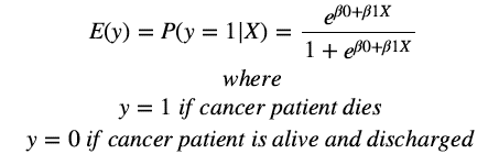
To fit the logistic model we use a method called maximum likelihood estimation.
Building the logistic model
Variables included in the study are as follows:
Stay_int = Number of days spent in ICU by cancer patients
Age = Age of cancer patient
Sex = Patient sex (male or female)
Type = Type of patient admission into ICU (elective, emergency or urgent)
We fit the full model with main exposure (time spent in ICU), age, sex and admission type:


From the output of the model, we see that type of admission is significant however no other variables are significant (p-value greater than the default value of α = 0.05 ). Therefore, we can go ahead and drop the sex variable.


From the model above, we see that the interaction between number of days spent in ICU and patient’s age in not significant as p-value greater than the default value of α = 0.05. Therefore, we can say that patient’s age is not an effect modifier for our main exposure (time spent in days in ICU for cancer patients).


From the output above, we can see that all the variables are now significant including our main exposure (number of days spent in ICU), cancer patient’s age, and type of admission (elective, emergency and urgent). Therefore, this is our final model.
We can do an anova to establish whether the non-interaction model is indeed a better model than the interaction
model.
We can confirm that the non-interaction model is better than the interaction model:


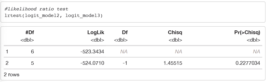
From the two outputs above, by using the Likelihood ratio test, we can see that the p-value = 0.2277 > α = 0.05 for △ G2 = 1.4552. Therefore, we fail to reject the null-hypothesis and hence, we can say that the main effects model is better than the interaction model. We should therefore choose the non-interaction model (logit_model3) as our best fit model. Since, the interaction is not significant between number of days spent in ICU and and age, we can say that there is no effect modification. Effect modification is when a variable that
differentially (positively and/or negatively) modifies the observed effect of a risk factor on a disease status.

We can test the full model using Wald’s test to check for the relationship between response and predictors.
Setting up our hypothesis:

From the output, the Wald χ2 = 7.4 with p-value = 0.0065. This indicates that the probability of patient mortality depends on at least one predictor at alpha = 0.05.
We can go ahead and calculate 95% the confidence intervals for the coefficients of our variables.
Confidence interval for the logit model is,

From the confidence interval, we see that none of the 95% confidence intervals capture 0 and hence we can say that the variables are significant.

To calculate the antilog for βi:


We can also check for confounding of variables in the model. A variable that can cause or prevent the outcome of interest and the effects cannot be distinguished from those of other factors being studied is said to be confounding. This happens when the association between the exposure and the outcome is obscured by a third variable or factor that:
a. Is associated with the exposure
b. Is associated or is independent factor for the outcome
Since our main exposure is time spent in ICU by cancer patients (in days), we can check to see if age is a confounder.

We find that after dropping age from our model the main exposure βDays spent in ICUchanges less than 10% (changes by 6.67%). Therefore, we can conclude that age is not confounding with our main exposure, days spent
in ICU by cancer patients.
Now, let us see if the type of admission is a confounder:

From the output above, we do see that days spent in ICU has a confounding effect with type of admission (whether elective, urgent or emergency). When admission variable is removed from the model, the main exposure βDays spent in ICU changes by more than 10% (changes by 26.7%). From this we can conclude that type of admission by cancer patients has a confounding effect with days spent in ICU.
betaStayint = 0.015020433. This indicates that an increase in days spent in ICU by a cancer patient is associated with an increase in the probability of patient mortality. To be more precise, a one-unit (day) increase in cancer patient stay at ICU is associated with an increase in the log odds of patient mortality by 0.0150 units.
expβ = 1.015 Stayint e0.015020433. Therefore, for every additional day spent in ICU, we estimate the odds ratio of mortality to be multiplied by about 1.015 i.e there is an increase of 1.5% [=(1-1.015)*100%] odds of cancer patient mortality.
betaAge = 0.006015989. This indicates that an increase in a cancer patients age is associated with an increase in the probability of patient mortality. To be more precise, a one unit increase in age (1 year) for a cancer patient is associated with increase in the log odds of patient mortality by 0.006 units.
expβ = = 1.0060341 Age e0.006015989. Therefore, for every increase in age by a year, we estimate the odds ratio of mortality to be multiplied by about 1.006 i.e there is an increase of 0.6% [=(1.0060-1)*100%] odds of patient mortality.
betaEmergency = 1.957784856. This indicates that a cancer patient admitted due to emergency admission is associated with an increase in patient mortality as compared to a patient admitted due to elective admission. To be more precise, a cancer patient admitted as an emergency admission is associated with an increase in log odds of patient mortality by 1.958 units.
expβ = = 7.083 Emergency e1.957784856. Therefore, if a cancer patient is admitted as an emergency admission, we estimate the odds ratio of mortality to be multiplied by about 7.083 i.e there is an increase of 608.3% [(7.083-1)*100] odds of patient mortality as compared to a patient admitted under elective admission.
betaUrgent = 1.659224184. This indicates that a cancer patient admitted due to urgency admission is associated with an increase in patient mortality as compared to a patient admitted due to elective admission. To be more precise, a cancer patient admitted as an emergency admission is associated with an increase in log odds of patient mortality by 1.660 units.
expβ = = 5.255 Urgent e1.659224184. Therefore, if a cancer patient is admitted as an urgent admission, we estimate the odds ratio of mortality to be multiplied by about 7.083 i.e there is an increase of 425.5% [(5.255-1)*100] odds of patient mortality as compared to a patient admitted under elective admission.
Graphical Distribution of the effect of time spent in ICU (in days) with cancer patient mortality.


The function ggsurvevents() [in survminer] calculates and plots the distribution for patient death events (both status = 0 and status = 1). As we can see from the output above, as cancer patients spend more days in ICU (time variable in x-axis), the ratio of deaths (delta = 1) to survivals (delta = 0) increases as shown by increased grey as compared to black area in the graph above.
Evaluating the logistic regression model
1. Deviance - The deviance is a measure of goodness of fit of a generalized linear model. The null deviance shows how well the response variable is predicted by the model that only includes the intercept. The residual deviance indicates how well the response is predicted by the model with independent variables. In our model, we have a value of 1208.6 on 1392 degrees of freedom. Including the independent variables (days spent in ICU, age,
and type of admission), decreased the deviance to 1048.1 on 1388 degrees of freedom, a significant reduction in deviance. The residual deviance has reduced by 160.5 points with a loss of 4 degrees of freedom.
2. AIC (Akaike Information Criteria) - The AIC provides a method for assessing the quality of the model through comparison or related models and is based on deviance. Our final model has an AIC value of 1058.1 and that is slightly less than the interaction model which has an AIC value of 1058.7. In general, model with a smaller AIC value is a better model.
3. ROC curve (Receiver Operating Characteristic) - The ROC curve is a plot to represent the true positive rate (sensitivity), the probability of predicting a real positive will be a positive, against false positive rate (1-specificity), the probability of predicting a real negative will be positive. A good model should be high on sensitivity and low on 1-specificity. It’s a rule that predicts most true positives will be a positive and few true negatives will be a positive.


We find that the AUC (Area under the curve) for our model is 0.738.
Hence we define our final logistic model as:


The predicted mortality probability for a 70 year old cancer patient admitted to emergency at the Beth Israel Deaconess Medical Centre between 2001 and 2012 is 0.23% if all else is kept constant. The predicted mortality for a 55 year old patient also admitted to emergency at Beth Israel Deaconess Medical Centre between 2001 and 2012 has a predicted mortality probability of 0.1744%, if all else is kept constant. This indicates that a 70 year old
patient in emergency type admission has a higher mortality probability than a 55 year old patient in elective admission type (a cancer patient that is both younger and is admitted under a different admission has a lower probability).
Survival Analysis
Kaplan Meier Curves helps understand the differences in survivorship between different cancer patients (males and females) and patients admitted as either elective, emergency or urgent.
The two most important measures in cancer studies include:
1. The time to death
2. The relapse-free survival time, which corresponds to the time between response to treatment and recurrence of the disease (also know as disease-free survival time and event-free survival time).
In this study, we are interested in exploring the time to event (patient mortality) for different cancer patient cohorts (male and female cancer patients) and cancer patients admitted to ICU under either elective, emergency and urgent admission.
Two related probabilities are used to describe survival data: the survival probability and the hazard probability. The survival probability, also known as the survivor function S(t), is the probability that an individual survives from the time origin (e.g admission to ICU) to a specified future time h(t). The hazard, denoted by, is the probability that an individual who is under observation at a time has an outcome of the event at that time. Thus, in contrast to the survivor function, which focuses on not having an event, the hazard function focuses on the event occurring.
The Kaplan-Meier (KM) method is a non-parametric method used to estimate the survival probability from observed survival times. The survival probability at time ti, S(ti), is calculated as follows:
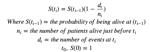
The estimated probability (S(t)) is a step function that changes in value only at the time of each event. Thus, we use the Kaplan-Meier survival curve, a plot of KM survival probability against time, as it provides a useful summary of the data that can be used to estimate measures such as mean survival time.
Therefore, we compute the survival analyses of cancer patients in MIMIC-III admitted under either elective, emergency and urgent admission. We subsequently use a Kaplan-Meier plot to summarize and visualize the results of the survival analysis.
Kaplan-Meier Curve to show Survival Analysis of cancer patients admitted as either elective, emergency or urgent admission.


From the Kaplan Meier curves above, we see some interesting results. For cancer patients that were admitted under emergency admission many more patients experiences the event (death) as compared to patients admitted under urgent or elective treatment. We also see that at around 40 days, emergency cancer patients have a 50% survival probability as compared to cancer patients admitted under elective surgery, who have a 50% survival
probability of about 75 days. For cancer patients admitted under urgent admission, there are fewer patients that experience the event however, it is also important to note that there are fewer patients in that cohort to begin with.
We see that the confidence interval are quite wide for cancer patients admitted under urgent admission, thus giving us a clue that the study contains very few participants. Interestingly, we also see widening of confidence intervals for elective cancer patients after around 30 days and emergency cancer patients at around 80 days, thus also indicating that the study contains very few participants at the respective time as the participants in the study
experience the event of interest (death) and the number of participants decrease as the study goes on.
Log-rank test.
Filtering data for elective and emergency patients in order to do a log rank test.

Performing the log-rank test.
The log rank test is the primary tool for the comparison of the survival estimates of two or more groups. The log rank test compares the entire survival experience between groups and can be thought of as a test of whether the survival curves are identical (overlapping) or not. It is designed particularly to detect a difference between survival curves which result when mortality in one group is higher than the corresponding one in the second group and the
ratio of these is constant over time. The log rank test is closely linked to the chi-square test statistic and compares observed to expected numbers of events at each point over the follow-up period. In our study, we have a cross over between the elective and urgent survival curves. Therefore, it would not be appropriate to conduct a log rank test to detect whether there is a difference between cancer patients admitted under elective admission
and those admitted under urgent admission. However, since we do not have a cross-over between elective and emergency admitted cancer patients, it would be beneficial and appropriate to filter the data and perform a logrank test for elective and emergency admitted cancer groups in order to test whether there is a difference between the two groups in terms of their respective survival curves.

From the output above, the value of chi-square statistic is 55.9 with 1 degrees of freedom and p-value is therefore 0.00000000000007 and hence we would reject the null-hypothesis in favour of the alternative hypothesis as 0.00000000000007 < 0.05 (default value of alpha). Thus, we would reject the null hypothesis that the survival estimate between emergency cancer patients and elective cancer patients is identical and therefore we could say
that the survival estimates between the elective and emergency patients is not identical and hence elective cancer patients can be said to fare better than emergency cancer patients.
Kaplan-Meier Curve to show Survival Analysis of Male and Female cancer patients.
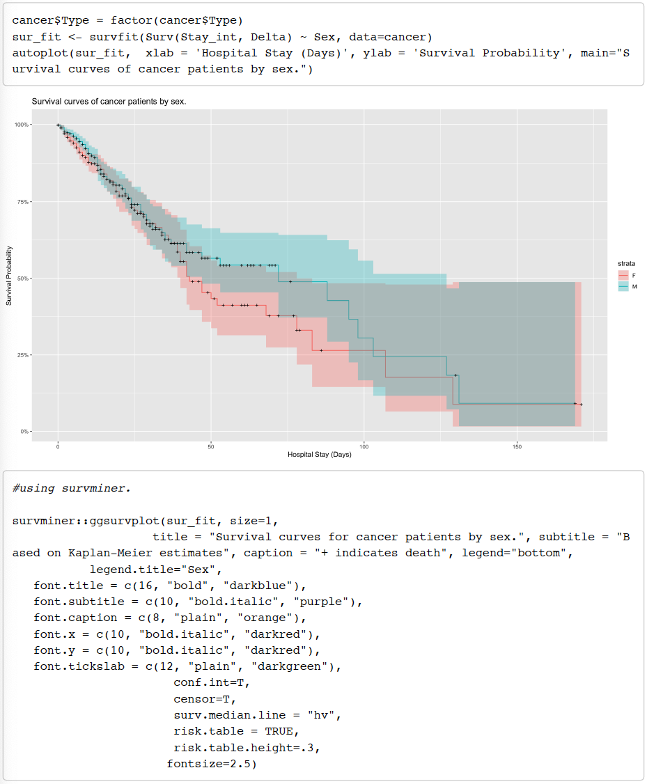

From the Kaplan Meier curves above, we see that both many male and female patients experience the event (death) starting almost from day 1 and continuing till day 40 whereby we see that the confidence intervals start to widen for both groups thus indicating that the study contains fewer patients after the 40 day mark as the participants in the study experience the event of interest and the number of participants decrease as the study
goes on. However, no conclusive results can be obtained from this Kaplan Meier model as we see that there is much crossing over between the two survivor curves and hence it would not be accurate to perform a log-rank test.
Cox Proportional Hazards Regression for Survival Analysis.
The Cox proportional-hazards model (Cox, 1972) is essentially a regression model commonly used statistical method in medical research for investigating and studying the association between the survival time of patients in a certain category and one or more explanatory variables. Cox proportional hazards regression analysis works for both quantitative as well as for categorical variables in our predictions. In clinical research and studies, there are
many situations, where several known quantities (known as covariates), potentially affect patient prognosis. The cox proportional-hazards model is one of the most important methods used for modelling survival analysis data.
For our analyses in regards to the survival of patients with some form of cancer, we will be looking at the effect of different types of surgery (if any) that a patient might undergo, while in the ICU over the time of stay in the hospital.
The Cox model is expressed by the hazard function denoted by h(t). Briefly, the hazard function can be interpreted as the risk of death or survival at time . It can be estimated as follows:

Where:

The h(t) is a hazard function which varies over time t as changes.
The Cox model can be written as a multiple linear regression of the logarithm of the hazard on the variables xs with the baseline hazard being an ‘intercept’ term that varies with time.
Generally, a value of greater than 0, or greater than 1, indicates that as the value of the covariate increases, the event hazard increases and the time length of survival decreases. Thus, in short it tells us that the covariate with HR>1 is positively associated with the event and negatively associated with the length of survival. When HR=0 there is no effect of that covariate on the event.

After describing the general Cox proportional hazard regression model, we will start looking at building our own model. For this we will work with the hypothesis we want to test, set a basic model and look for effects of different predictors on the model. Important notion to consider are whether there are any a priori hypotheses to be tested and whether a multiple variable model is even needed. Since, there is often a considerable amount of variability
between subjects in a medical study, finding a parsimonious model that is relevant to the outcome of interest is very important.
Testing the hypothesis for distribution of time to death are the same for different surgery types experienced by the cancer patients.
With this, we will now define our basic model. Our significance level ( ) is set at 0.05. We will be relying on the Wald Statistic values (z) in our summary outputs to determine the significance of the variable in the model. The Wald statistic evaluates, whether the beta ( ) coefficient of a given variable is statistically significantly different
from 0.
The covariates that we are interested in studying that may potentially affect cancer patient prognosis from a clinical study standpoint are:
Surgery (main-exposure for the study) = Type of surgery patient surgery (cardiac surgery, neurological surgery, general surgery, thoracic surgery and vascular surgery).
Sex = Male and female patients in MIMIC-III data
Age = Patient’s age
Type = Type of ICU admission (either elective, emergency or urgent). This is mainly chosen by us because generally to study such patient cohort, we have some form of severity index.
Since, the MIMIC data was missing it, we felt that this variable might be a close option to test severity of cancer patients after their surgery.
Note: Hospital (ICU) stay time in our analysis over which the outcome is measured is set to begin after the patient undergoes the surgery. (Details discussed in limitations later)
We first set our reference level to “no-surgery” as surgery is our main exposure and we want to primarily compare patient prognosis for cancer patients that have undergone surgery to cancer patients that have not undergone any surgery.
Building a univariate cox regression with only our main exposure (type of surgery).
We now build a univariate cox model with our main exposure as type of surgery.


From the output above, we see that the p-value for all three overall tests (likelihood ratio test, Wald and logrank) are significant, indicating that the model is significant. These tests evaluate the omnibus null hypothesis that all βs the are 0. From our model, the omnibus null hypothesis is soundly rejected as p-value is less than the default value of α = 0.05. The Wald statistic evaluates, whether β the coefficient of our variable (type of surgery) is statistically significantly different from 0. Therefore, from the output, we can conclude that the two types of surgeries are significant; neurological and general surgery.
We now proceed to a multivariate cox regression analysis to see how our other variables jointly impact survival. Therefore, we will add age, sex and type of admission to our main exposure (type of surgery). We also add interaction term to see if there is an effect modification between type of surgery that cancer patient undergoes and age.
Multivariate Cox Regression Analysis including interaction between age and type of surgery to see how factors jointly impact survival.

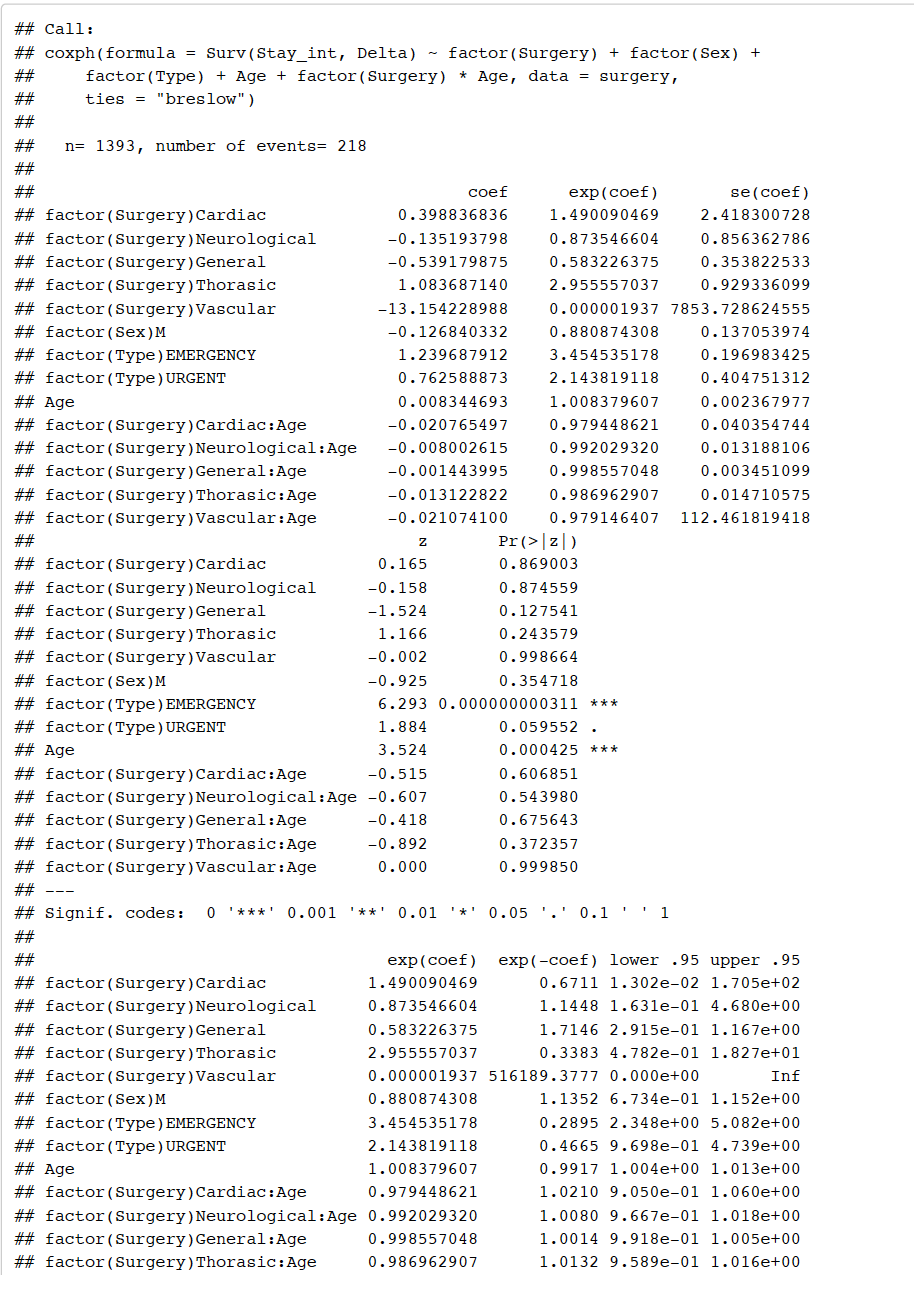

From the output above, we see that interaction between type of surgery and age is not significant as p-value > 0.05 (default value of alpha). Therefore, we drop the interaction from our model.
Multivariate Cox Regression Analysis without interaction.


From the output, we see that after dropping interaction term, neurological and general surgery remain significant however if a patient was admitted under emergency type admission and the patients age now becomes significant as p-value < 0.05 (default value of alpha). The p-value of a patient admitted as emergency admission is 0.000000000157, with a hazard ratio of exp(1.2633666550) = 3.537, indicating a strong relationship between
cancer patients admitted as emergency admission and increased risk of mortality. The p-value of a cancer patients age is 0.000066922764, with a hazard ratio of exp(0.0068663694) = 1.0068, indicating a strong relationship between cancer patients age and increased risk of mortality.
We can perform an anova to compare the models with interaction and without interaction. Testing the hypothesis.

From the output above, we see p-value 0.7989 > default value of alpha at 0.05. Therefore, we accept the nullhypothesis and we can say that there is evidence to suggest that the model without interaction is a better model.
We now drop sex from our model as it was found to be insignificant in the previous model.
Multivariate Cox Regression Analysis without sex variable

From the output above, we can see that neurological and general surgery remain significant and patient’s age and emergency admission remain significant and urgent emergency now also becomes significant. We can subsequently check to see if dropping the sex variable is a better model than the model with sex included.


From the output above, we see that p-value 0.3554 > 0.05 (default value of alpha) and hence we accept the null hypothesis and we say that there is evidence to suggest that the model without sex is a better model. Therefore, we proceed with the model without sex.
We also check if there is an interaction between type of surgery and type of admission:
Checking for interaction between type of surgery and type of admission multivariate cox regression.


From the output above, we see that non of the interactions are significant as p-values are more than the default value of alpha at 0.05. Furthermore, we also see that including interactions makes neurological and general surgery and age insignificant. We can go ahead and confirm that the non-interaction model (effect modification between type of surgery and type of admission) is not better than the non-interaction model.
Anova to show model without interaction is better than model with interaction between type of surgery and type of admission:

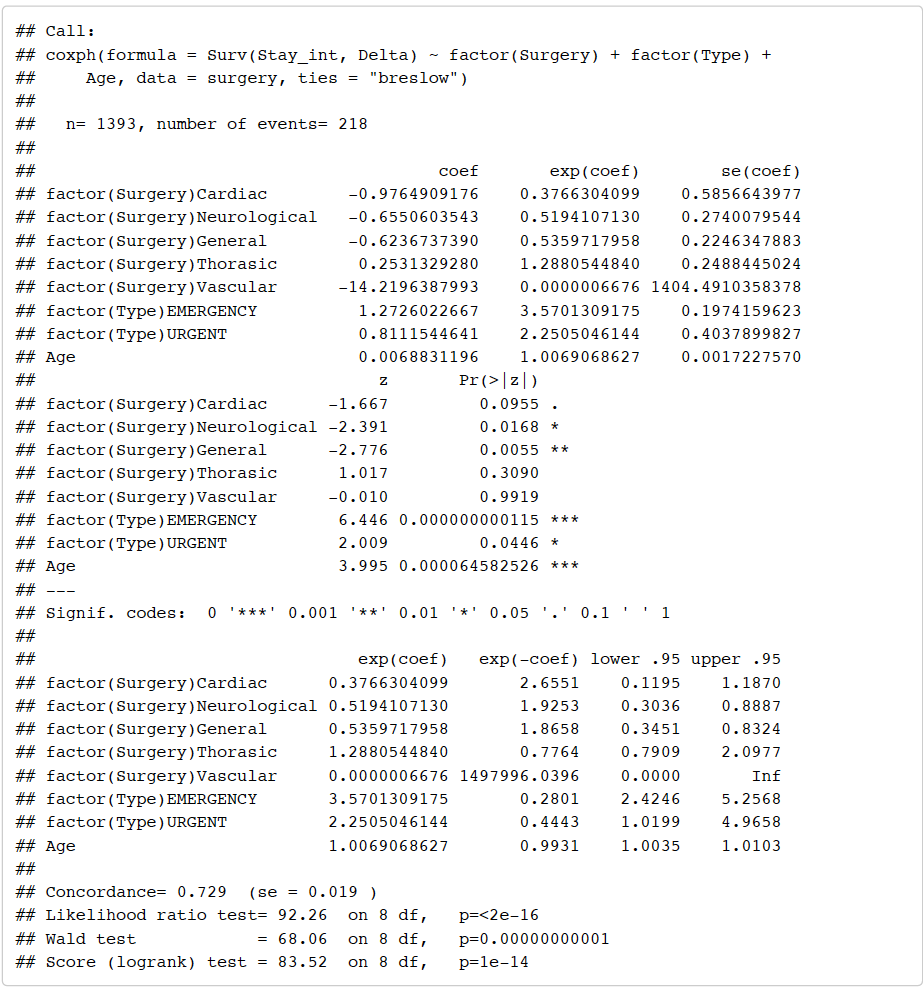
Final Multivariate Cox Regression with significant variable.

From the output of the final model, we see that neurological surgery, general surgery, emergency admission, urgent admission and patient age are all significant (p-value less than default value of alpha at 0.05. The p-value for all three overall tests (likelihood, Wald and logrank test) are significant, indicating that the model is significant.
Here we need to now check for assumptions to ensure our model meets the Cox PH assumption. Thus, we move into the assumption testing.
Checking for proportional hazard assumption.
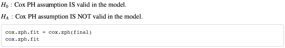
For the proportional hazards to be met, the p-values for Age, Surgery (type of surgery), Type (type of admission) and the global test must be insignificant. Using the cox.zph function, we build the following table. Here we test the hypothesis that:

From the summary table above, two covariates are statistically insignificant and even the global test is insignificant. But one level of the covariate, type of admission (Type) does not meet the Cox PH assumption. Since, the interaction above as well was not significant, we cannot introduce interactions, as sometimes it makes the proportional hazard (PH) assumption true.
Note: Something we did here to deal with this particular issue is we tried changing reference level for type of admission (since it is categorical). The hazards may be proportional when compared to one reference category but not the other. Hence, by switching the reference categories, we wanted to see which category might drive the PH assumption to be true.
After testing different methods to deal with for the assumption to be met, we were not able to get the covariate to meet the PH assumption. Since, the switching of reference levels did not help us solve our problem, this indicated that the hazards is not proportional for this particular covariates, i.e. different hazards at different time points for this covariate. If the covariate was continuous in nature, we could have applied something called as stratification
of the model over different time points to be able to meet the PH assumption. Since, Type being a categorical variable, we could not make the stratification happen.
After careful examination and looking at general clinical studies closely related to the MIMIC-III data, we decided to drop the variable for types of admission (Type) as it is not a critical predictor of survival over time after patient
has had their surgery. Additionally, the variable is not a biological or medical feature which would be critical in any prediction, rather it is an administrative variable used for the stratification of admission class to ICU.
Final model


Cox PH model assumption test
Scaled Schoenfeld Residuals
Let us test again the assumption of PH for our model using the previous hypothesis.

Comparing to our previous model that we had fit and tested for assumptions, this model meets all our PH assumption. Since, the global and individual test is highly insignificant, we fail to reject the null hypothesis and conclude from our hypothesis that this final model of ours which includes age as a predictor in the model with main exposure as type of surgery, meets all the PH assumptions, i.e. all the hazards are proportional for all the
covariates. Hence, we can assume the proportional hazards in the model.
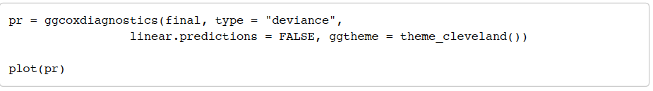
For testing the assumption and checking the proportional hazards graphically, we can plot a series of graphs of scaled Schoenfeld residuals for each covariate against time of observation.

In the plot above, we have a solid smooth line and the dotted lines around the smoothing fit which represents a +/- standard-error band around that fit. From the graphical inspection, we see no patterns over time for Age and for type of surgery (Surgery). Remember, Surgery has six levels and we see a sharp deviation from the fit line for Thorasic and Vascular surgery. This means, we might have varying values for their over time. βs If we also see the
number of observation, there seems to be sparse observation of patients as we move right on the x-axis (i.e. stay longer in ICU) and that causes the confidence bands to deviate at the ends. Nonetheless, we can confirm that the assumption of proportional hazard is met.

Interpretations.
Since, we checked for the assumption and established that the final model is valid, here we do the following interpretations.
A note here, a positive sign means that the hazard (risk of death) is higher, and thus the prognosis becomes worse, for subjects with higher values of that variable.
Age: Looking at βage = 0.0058the indicates that as age increases, the risk of death or hazard increases. Thus, age has a significant effect on cancer patients in our data. The hazard ratio for age i.e., exp(βage) = 1.0058 indicates that age increases the hazard of death by a factor of 1.01 as compared to a lower age. Example, a person of age 55 is 1% [ (1.01-1)*100 ] more likely prone to death or has hazard ratio of 1.01 compared to someone of age 54.
Surgery: Remembering that we have 6 levels for surgery and reference level being None or no surgery. Thus, each surgery type has following effect:
Cardiac Surgery: βcardiac surgery = −1.2394 indicates that patients who have cardiac surgery have lower risk of death than those patients who do not have any surgery. The hazard ratio exp(βcaridac surgery ) = 0.2895, means cardiac surgery has lower risk of death by a factor of 0.2895 or reduces the risk of death by 71.05% compared to patient who did not undergo surgery. We can also be 95% confident that the risk of death after cardiac surgery is atleast 0.0916 to atmost 0.915 times compared to the risk of death from no surgery at all (values from summary table).
Neurological Surgery: βneurological surgery = −0.8863 indicates that patients who undergo neurological surgery have lower risk of death than those patients who do not have any surgery. The hazard ratio exp(βneurological surgery ) = 0.4122, means neurological surgery reduces the risk of death by a factor of 0.4121 or 58.79%.
General Surgery: βgeneral surgery = −0.9797 indicates that patients who undergo general surgery have lower risk of death than those patients who do not have any surgery. The hazard ratio exp(βgeneral surgery ) = 0.3754, means general surgery reduces the risk of death by a factor of 0.3754 or 62.46%.
Thorasic Surgery: βthorasic surgery = −0.2215 indicates that patients who undergo thorasic surgery have lower risk of death than those patients who do not have any surgery. The hazard ratio exp(βthorasic surgery ) = 0.8013, means neurological surgery reduces the risk of death by a factor of 0.8012 or 19.88%.
Vascular Surgery: βvascular surgery = −14.4256 indicates that patients who undergo vascular surgery have lower risk of death than those patients who do not have any surgery. The hazard ratio exp(βvascular surgery ) = 0.000000543, means vascular surgery reduces the risk of death by a factor of 0.000000543 or 99.9999457%.
Testing for influential subjects in the data.
In the Cox PH regression model, we can test for influential outliers or observations in our data.

The above plots show that comparing the magnitude of the largest dfbeta values to the regression coefficients suggests that none of the patients is highly influential individually, even though some of the dfbeta values for cardiac and vascular are large compared with the other variables
Testing for the outliers using deviance residuals.
We can check for the outliers by visualizing the deviance residuals as well. The deviance residual is a normalized transformation of the martingale residual. These residuals should be roughly symmetrically distributed about zero with a standard deviation of one.

From this plot we check for deviance for the residuals of our observations. Most residuals are spread symmetrically around the zero fit line. The values over zero are related to patients who died before the expected survival time. Values below zero are related to patients who lived longer than expected survival time.
Testing for non-linearity for Age.
Often, we assume that continuous covariates have a linear form. However, this assumption should be checked. Plotting the Martingale residuals against continuous covariates is a common approach used to detect nonlinearity. For a given continuous covariate, patterns in the plot may suggest that the variable is not properly fit. Non-linearity is not an issue for categorical variables, so we only examine plots of martingale residuals and partial
residuals against a continuous variable.
We will check for linearity assumption for the model by the following plot.


From the plot above, we see that there might be some non-linearity present within our continuous covariate. We also included a log transformation for age to see its effect as well.
Results
From the detailed analysis carried above for the 1394 unique cancer patients in the dataset we created from the larger MIMIC-III dataset, we investigated and discovered the following interesting findings.
In context to predict the outcome of an event i.e. death or discharge, we found that the time spent in ICU was a significant predictor. We wanted to analyze whether time spent in ICU had an effect on the outcome and it was an important feature in the model. We also deduced that the type of admission under which the cancer patients were
categorized also played a significant role, and was accompanied by age of the patient in predicting the likely outcome of survival or death.
For the survival analysis conducted on the type of admission under which the cancer patient was admitted in the ICU, we found that the patients who were admitted under the emergency category were more likely to experience the event of death than those in elective or urgent category. Also, the median hospital stay time in the emergency
admission category was approximately forty days against the other categories which had median survival time of seventy days. Also, comparing the sex of the patient in the survival analysis tells us, if the patient is female, the median survival or stay in the ICU was approximately forty days, whereas for males the median length of stay was
around 75 days.
Lastly, testing and analyzing the Cox Proportional Hazard Regression Model, where we were interested in seeing whether time has an effect on the outcome of death or discharge from ICU for different types of surgeries experienced by the patients. We found out that, infact surgery does improve the survival rate of the cancer patients over time after the surgery, compared to those who did not undergo any surgery. So surgery does have a
significant effect on the survival of patients in our data. From the model, we also did find age to be a significant predictor for type of surgery and its effect on the overall outcome.
Discussion and Conclusions
The results above contribute to the body of literature suggesting that some form of surgery does have a benefit or good effect on the survival of cancer patient. We described the hypothesis at the beginning and conducted our analysis towards testing it. We conclude that cancer patients, who have some form of surgery and after spending
some time in the ICU for recovery, do have favorable outcome i.e. have better survival rate compared to those patients who did not have a surgery. When we started off with the hypothesis, we expected to see improvements
in the survival of cancer patients over an observed time period as surgeries are meant to alleviate suffering (palliative) or to remove the tumor in affected areas (preventative) of patients from a given cancer diagnosis. The conclusion of our results were very much similar to our expectation.
But in general, our expectation and results versus some other theories that have been in debate might influence the health studies differently. In general practice, the expectation of lower survival rate in patients who undergo surgery is quite prevalent in the medical field. This could be due to numerous factors and might have effects differently from different patients. This could depend on age, diagnosis, genetic build, sex, etc. There could be
external factors such as socio-economic effect on the patient, health care cost, medical aid, etc. These form more of a non-biological factors for accounting in survival of a patient, in general. While studying our data and investigating our model, we realized few weakness and limitation that come from MIMIC-III dataset.
Limitations
Though our approach showed strong performance for several tasks in this dataset, this method currently has limitations in terms of generalization. These limitations might hinder or provide diluted results in further analysis and future studies. Following were some key limitations we noted while working on the dataset.
1. MIMIC-III data has the time records for different variables associated with time, censored or modified to show different time frame for potential privacy reasons. This made it challenging for us to triangulate exactly when in realistic experience were the hospital stays and events for the patients in the dataset measured or recorded.
2. Due to this reason, we were also not able to accurately factor in the time and period in which a patient had undergone a specific surgery. Due to this, we made an assumption of the surgeries to have occurred before the time spent by patients in the ICU.
3. After reading few clinical research papers, we learned that a presence of some of emergency severity index (ESI) (Louden et al.) is a common practice in medical records. The index explains the severity of an illness in the patient group between patients. This specific index is particularly viable and important for patients visiting ICU. MIMIC-III dataset, does not have such a feature available in it. To proxy this, we used type of admission to ICU, but it does not bare much evidence or value as an actual index might do. Also, type of
admission is largely used to stratify patient group for administration purposes. In such future studies as the one done by us, having a severity index, would be a good predictor to use for adjusting the effect of surgeries in survival analysis. To study between our different cancer patients, addition of a form of severity index would enhance the model to provide better results.
4. Our model also has more than 700 different cancer diagnosis. It was not feasible to run the model with these many different diagnosis, some being recorded with errors or duplication for same diagnosis with different nomenclature system. This might make the analysis diluted and introduce errors in the results. Further along, some cancer has worse prognosis than the other. We did not account for different cancer types in our model but might be applicable for a modified analysis.
5. Cancer survivors suffer from many comorbid conditions that could be of great influence on their health and the effect on cancer itself. Conditions such as hypertension, hyperlipidemia, osteoarthritis, hypothyroidism, diabetes mellitus, etc. are of significant health implications and could have significant prevalence in cancer patients. This information is not easily interpretable due to amount of records in the MIMIC-III dataset with ICD-9 coding, and would need a lot more computation power than a simple laptop. Having these
comorbidities readily available for the patients in the data, would help analyze their effect to our outcome in the hypothesis. This could be a consideration in further studies to apply more computation power (different programming language such as linux or C++) to access the information and decode it for the actual comorbidities rather than ICD-9 coding.
Inclusion and presence of some variables related to lab work and readings associated to blood pressure, diabetes, creatinine, etc. would be highly valuable and could be significant in our future modeling. Although the file related to blood work was available in the MIMIC data, the sheer volume and size of it, led to the file not being able to read with methods and tools available to us. Making the data more concise for elementary studies would be invaluable.
References
1. Newell, Christopher, Barbara Ramage, Alberto Nettel-Aguirre, Ion Robu, and Aneal Khan. “Peak Jump Power Reflects the Degree of Ambulatory Ability in Patients with Mitochondrial and Other Rare Diseases.” In JIMD Reports, Volume 33, pp. 79-86. Springer, Berlin, Heidelberg, 2016.
2. Beaulieu-Jones, Brett K., Patryk Orzechowski, and Jason H. Moore. “Mapping patient trajectories using longitudinal extraction and deep learning in the MIMIC-III Critical Care Database.” In PSB, pp. 123-132. 2018.
3. Rich, Jason T., J. Gail Neely, Randal C. Paniello, Courtney CJ Voelker, Brian Nussenbaum, and Eric W. Wang. “A practical guide to understanding Kaplan-Meier curves.” Otolaryngology—Head and Neck Surgery 143, no. 3 (2010): 331-336.
4. Chen, Herbert, Jeffrey M. Hardacre, Ali Uzar, John L. Cameron, and Michael A. Choti. “Isolated liver metastases from neuroendocrine tumors: does resection prolong survival?.” Journal of the American College of Surgeons 187, no. 1 (1998): 88-92.
5. Louden, B. Asher, Daniel J. Pearce, Wei Lang, and Steven R. Feldman. “A Simplified Psoriasis Area Severity Index (SPASI) for rating psoriasis severity in clinic patients.” Dermatology online journal 10, no. 2 (2004): 7-7.
6. Roy, Satyajeet, Shirisha Vallepu, Cristian Barrios, and Krystal Hunter. “Comparison of comorbid condition between cancer survivors and age-matched patients without cancer.” Journal of clinical medicine research 10, no. 12 (2018): 911.
Appendix
The data wrangling and subsetting of cancer patients from MIMIC-III data was completed in Python. The Jupyter notebook is attached separately to see the methods and steps taken to construct the final data file for our use which is “Cancer_Surgery.csv”.
The code chunk for investigating general descriptive statistics for the data is attached below.


Comments